Next: 5. New Identifications Up: 4. Proposed algorithms and Previous: 4. Proposed algorithms and
![]()
![]()
![]()
Next: 5.
New Identifications Up: 4.
Proposed algorithms and Previous: 4.
Proposed algorithms and
To test the proposed algorithm, and also to tune the control values of the different distances to be used to propose identifications, we have selected a set of already identified orbits with the following criteria:
 |
We have used a set of 100 examples, satisfying the above conditions, for which observational data are available from the Minor Planet Center Extended Computer Service. For all, we have recomputed the best fit orbit and the normal/covariance matrices for each one of the two arcs containing observations from a single opposition.
These nominal solutions, and the corresponding matrices, are computed
for the epoch of the last observation in each arc. Then we have propagated
all the orbital elements, and all the normal and covariance matrices, to
a common epoch (we have used ![]() ;
for the dependence of the results upon this date, see Section 5). This
propagation was done with accurate numerical solutions of the
;
for the dependence of the results upon this date, see Section 5). This
propagation was done with accurate numerical solutions of the ![]() -body
equations of motion, and of their variational equations, while the normal
and covariance matrices were both propagated by means of equations (4),
with no further inversions after the single one performed at the observations
epoch.
-body
equations of motion, and of their variational equations, while the normal
and covariance matrices were both propagated by means of equations (4),
with no further inversions after the single one performed at the observations
epoch.
With all the state vectors and normal/covariance matrices referred to
the same epoch, the algorithms of Section 2 can be applied, and we have
used them according to the same procedure outlined at the beginning of
this Section, namely by computing ![]() ,
,
![]() and
and ![]() for each test couple, formed by two observed arcs known to be of the same
asteroid.
for each test couple, formed by two observed arcs known to be of the same
asteroid.
 |
The results of the computation of our three metrics are shown in the
histograms of Figures 2-4.
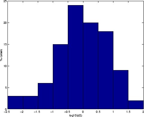
In Figure 2 we show the results
for the inclination-only distance ![]() ;
it is apparent that this distance has always a low value,
;
it is apparent that this distance has always a low value, ![]() in
in ![]() of the test cases,
of the test cases, ![]() in
in ![]() ,
with a maximum value of
,
with a maximum value of ![]() .
This is, however, a loose criterion which can be used only as a preliminary
filter, since in a large catalog with tens of thousands of orbits it would
be satisfied by millions of couples.
.
This is, however, a loose criterion which can be used only as a preliminary
filter, since in a large catalog with tens of thousands of orbits it would
be satisfied by millions of couples.
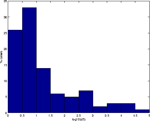
The distance ![]() being small is obviously a much stronger constraint on the couples of orbits
to be identified. Indeed it has a small value for many of the actually
identified orbits:
being small is obviously a much stronger constraint on the couples of orbits
to be identified. Indeed it has a small value for many of the actually
identified orbits: ![]() in
in ![]() of the test cases,
of the test cases, ![]() in
in ![]() .
It has, however, as shown in figure 3,
a moderate value in a number of cases:
.
It has, however, as shown in figure 3,
a moderate value in a number of cases: ![]() in
in ![]() of the cases, and an even larger value in
of the cases, and an even larger value in ![]() .
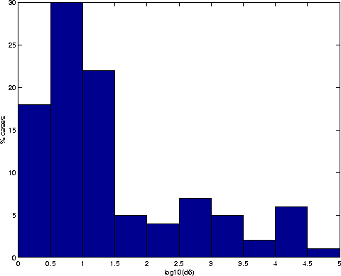
The distance
.
The distance ![]() is the one associated with the fully linear identification algorithm. Its
value is always larger than that of
is the one associated with the fully linear identification algorithm. Its
value is always larger than that of ![]() (this is just an example of the property
(this is just an example of the property ![]() proven in Section 2.3). Nevertheless, the value of
proven in Section 2.3). Nevertheless, the value of ![]() is low in most cases:
is low in most cases: ![]() in
in ![]() of our test sample; a low to moderate value
of our test sample; a low to moderate value ![]() covers
covers ![]() of the cases, as shown in Figure 4.
of the cases, as shown in Figure 4.
 |
A final test is based upon equation (2),
proposing two different formulas to compute the matrix ![]() ,
therefore
,
therefore ![]() ,
therefore the identification metrics. These two formulas would give identical
results in exact arithmetic, but are susceptible to give discordant results
when the normal matrices have very large conditioning numbers. The alternative
values for both
,
therefore the identification metrics. These two formulas would give identical
results in exact arithmetic, but are susceptible to give discordant results
when the normal matrices have very large conditioning numbers. The alternative
values for both ![]() and
and ![]() are
essentially identical (differences less than
are
essentially identical (differences less than ![]() )
in all cases, while for
)
in all cases, while for ![]() the difference are larger than
the difference are larger than ![]() of the value of
of the value of ![]() in
in ![]() of the cases. This is not unexpected: the full covariance matrix (also
the normal matrix) has a conditioning number growing with the time elapsed
after the observations, as it can be seen already from the 2-body approximation
of Paper I, Section 4.1; the reduced
of the cases. This is not unexpected: the full covariance matrix (also
the normal matrix) has a conditioning number growing with the time elapsed
after the observations, as it can be seen already from the 2-body approximation
of Paper I, Section 4.1; the reduced ![]() matrix does not have this property. Anyway the difference between the two
values is not really important in any of the test cases.
matrix does not have this property. Anyway the difference between the two
values is not really important in any of the test cases.
Another important test of our identification algorithm is the following.
The theory outlined in Section 2 does not only provide a minimum identification
penalty, but also a first guess for the orbit resulting from the
identification. The full linear algorithm computes a complete set of orbital
elements (![]() in the notations used in Section 2.1) which is the best solution in the
linear approximation, and should be used as starting value for an iterative
differential correction procedure, including all the observations from
both arcs.
in the notations used in Section 2.1) which is the best solution in the
linear approximation, and should be used as starting value for an iterative
differential correction procedure, including all the observations from
both arcs.
On the contrary, the restricted identification procedure provides only
a first guess for the orbital elements in the selected subspace (![]() in the notations used in Section 2.2). For the reasons already discussed,
this procedure does not provide a first guess for the elements not included
in the vector
in the notations used in Section 2.2). For the reasons already discussed,
this procedure does not provide a first guess for the elements not included
in the vector ![]() .
Thus, the identification based only upon the two elements
.
Thus, the identification based only upon the two elements ![]() does not provide a useful first guess, and the procedure based upon five
orbital elements provides a first guess for all the elements but the mean
longitude
does not provide a useful first guess, and the procedure based upon five
orbital elements provides a first guess for all the elements but the mean
longitude ![]() .
.
A simple minded procedure could be to devise some first guess ![]() by a procedure which does not take into account the uncertainty of the
two separate solutions for the two arcs, e.g.
by a procedure which does not take into account the uncertainty of the
two separate solutions for the two arcs, e.g. ![]() could be just the mean of the two values resulting from the two separate
arc solutions for the same epoch
could be just the mean of the two values resulting from the two separate
arc solutions for the same epoch ![]() (note that the average of two angles is not the average of their principal
values, but needs to be done with some care to avoid a mistake by
(note that the average of two angles is not the average of their principal
values, but needs to be done with some care to avoid a mistake by ![]() ).
).
As it could have been expected, this method to compute a first guess
is not very successful: the differential correction iterative procedure
converges to the identification orbit for only ![]() of the cases. But it can be valuable in cases where the
of the cases. But it can be valuable in cases where the ![]() is not useful due to very large uncertainty in
is not useful due to very large uncertainty in ![]() .
In fact, if the marginal uncertainty in
.
In fact, if the marginal uncertainty in ![]() is more than one revolution the
is more than one revolution the ![]() computation
can actually return more than one value, because the difference in
computation
can actually return more than one value, because the difference in ![]() can contain integer multiples of
can contain integer multiples of ![]() .
In these cases we use the result with the lowest
.
In these cases we use the result with the lowest ![]() ,
but the reliability of the test in these cases is dubious.
,
but the reliability of the test in these cases is dubious.
Then the real test of the quality of the linear identification algorithm
is to try to achieve convergence of the iterative differential corrections
procedure, using as starting point the ![]() set of orbital elements suggested by the algorithm as best solution in
the linear approximation. We have performed this test, and found convergence
to the identification orbit in
set of orbital elements suggested by the algorithm as best solution in
the linear approximation. We have performed this test, and found convergence
to the identification orbit in ![]() of the cases.
of the cases.
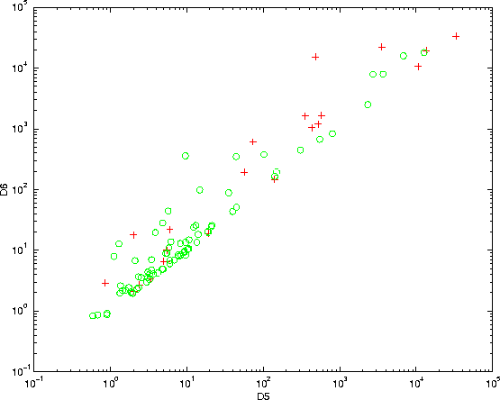 |
The results of these tests on the convergence of differential corrections
are summarized in Figure 5; the
crosses indicate the cases in which the convergence failed, when starting
from the ![]() guess; in all these cases, however, the full algorithm starting from
guess; in all these cases, however, the full algorithm starting from ![]() succeeded, with only one exception, which is indicated by the cross at
the top right of the Figure, with values of both
succeeded, with only one exception, which is indicated by the cross at
the top right of the Figure, with values of both ![]() and
and ![]() above
above
![]() . Even in this
isolated case, the differential corrections algorithm converged when the
first guess was the set of interpolated elements obtained with the algorithm
proposed in [Sansaturio et al. 1996].
. Even in this
isolated case, the differential corrections algorithm converged when the
first guess was the set of interpolated elements obtained with the algorithm
proposed in [Sansaturio et al. 1996].