3.2 Nonlinearity 3. Problems with the 3. Problems with the

   
3.1 Bad conditioning

In order to test and tune our algorithms, even before having access to the full dataset of observations, we have used an orbit catalog provided by Lowell Observatory containing the normal matrices $C$ for $37\,569$ asteroid orbits. Each $C$ had been computed by fitting an orbit to the observations at some central epoch $t_0$ near the center of the observation time span (E. Bowell, private communication, 1998; for a public domain version: ftp://ftp.lowell.edu/pub/elgb).

A positive-definite matrix has all the eigenvalues positive. This definition is computationally meaningful only provided the conditioning number of the matrix (the ratio of the largest to the smallest eigenvalue) is not larger than the inverse of the machine accuracy or relative rounding off error (typically $\simeq10^{-16}$).

To assess how severe the conditioning problem is we have computed all the eigenvalues of all the normal matrices of the Lowell catalog, and found $37\,544$ positive-definite matrices. In $25$ cases, however, there is at least one negative eigenvalue (in $2$ of these cases there are two negative eigenvalues).

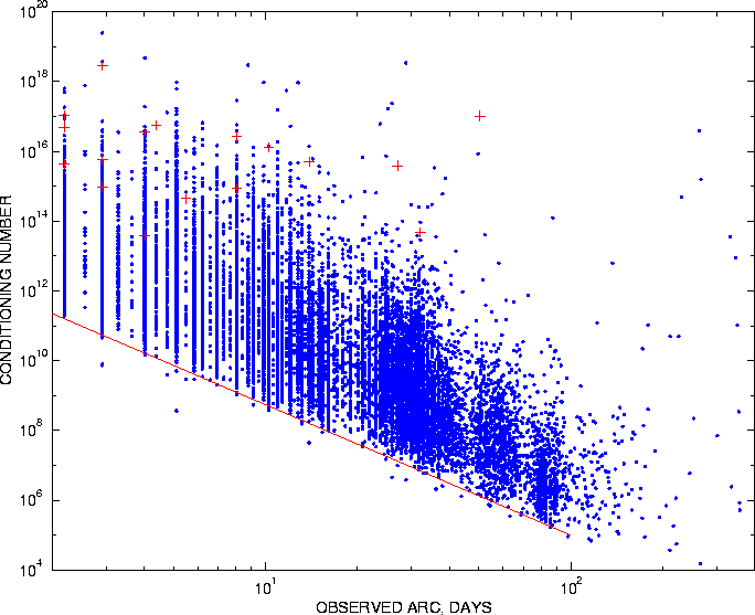
Figure 1 shows the logarithm (in base 10) of the observed arc (days) versus the logarithm of the conditioning number $\lambda_6/\lambda_1$; only the asteroids observed for less than one year are shown. The matrices with conditioning number close to, or even greater than, $10^{16}$ are ``numerically singular'' and can provide information only if handled with a very stable algorithm. For the $25$ cases with negative eigenvalues, the ratios $\lambda_6/\vert\lambda_1\vert$ between the largest positive and the largest absolute value of a negative eigenvalue are marked with crosses in Figure 1. The negative eigenvalues appear only in matrices which are anyway poorly conditioned, to the point that even the matrix multiplication $B^TB$ results in large rounding off errors. The concentration of the badly conditioned and even nonpositive-definite matrices in the cases where the observed arc is less than a month is apparent.

  

The covariance matrices provided by the Lowell Observatory are entirely suitable for the purposes for which they are used, that is differential correction and linearized ephemeris uncertainty. Indeed, for their purposes the less that linearity applies, the less important the accuracy of the covariance. Conversely, for our problem it is imperative that the worst cases have highly accurate uncertainty predictions in order to extend the linear theory as far as possible.

The number of badly conditioned matrices for the elements determined at the central epoch is large, but there are still enough matrices for which inversion is not a problem, provided a stable numerical method is used. We use the Cholesky algorithm, which allows one to perform the inversion of a matrix with conditioning number $w$ by means of the inversion of an auxiliary matrix with conditioning number $\simeq\sqrt{w}$; the failures of this inversion are indeed rare.

The bad conditioning problem is becoming much worse if the normal and covariance matrices are propagated to a different epoch $t$ (see Paper I, Section 2.4). The propagation equations contain the state transition matrices: if $X_0,C_0,\Gamma_0$ are at epoch $t_0$, and $X,C_t,\Gamma_t$ are at epoch $t$ then

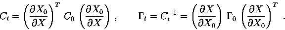$$C_t=\left({\displaystyle \partial X_0 \over \displaystyle \p......style \partial X \over \displaystyle \partial X_0}\right)^T\ .$$ (4)

From a 2-body approximation (see Paper I, Section 4.1) it is apparent that, even without close approaches, the conditioning number goes to infinity as $t\to + \infty$ in a quadratic way. Thus the inversion $\Gamma=C^{-1}$ should always be performed only for the central epoch, when the conditioning is as good as it can get; it is numerical suicide to wait until the conditioning number gets worse to perform an inversion.

The normal and covariance matrices need to be propagated to a common epoch if two orbits have to be compared for a possible identification; the best strategy is to propagate both of them separately by the matrix multiplications of the above formulae. Since this requires one to solve both the equations of motion and the variational equation accurately, it is a computationally intensive task; one may wonder if it is possible to use a simplified 2-body propagation. The answer to this question is definitely negative; this can be shown by comparing the eigenvalues of the matrices propagated with different approximations.

All these cautions have been used in the computations for the tests described in this paper, and are incorporated in our free software. As a result, in the test of Section 4 there are no cases in which the identification algorithm fails because of noninvertible and/or nonpositive-definite matrices.

3.2 Nonlinearity 3. Problems with the 3. Problems with the